Generating priors from historical data

Note, you can find the original Jupyter notebooks used to generate the plots in this post in my forecasts repo in the Foretell folder. The file is 20201118_value_of_Chinese_semiconductor-imports.ipynb, and there is a PDF printout of the file for ease of viewing

I have recently started forecasting on CSET’s Foretell platform. I’ve been interested in forecasting for a while, but I’ve always gotten stuck on where to start. The advice that most people seem to give (including Foretell’s own tutorial) is to start with a base rate (aka an “outside view”) and then update it using the specifics of the situation you are forecasting (aka an “inside view”). The problem I’ve had with this is that I generally have neither and inside view nor an outside view for most forecasts. I generally just come in with a uniform prior, thinking that all the options of the forecast are equally likely. In this post I’ll explain my first step to go beyond this “uniform prior” forecast.

One nice thing about Foretell’s questions is sometimes they provide data from which one can construct a base rate. One example of this is the question What will be the value, in dollars, of all Chinese imports of semiconductor manufacturing equipment in 2021? The “answer” to this question takes the form of your confidence that this dollar value will fall within the ranges (in units of billion USD) {[0, 20], (20, 30], (30, 40], (40, 50], (50, $\infty$)}

If you click “Show background information” below the question, they provide nine years’ worth of data measuring exactly this quantity.

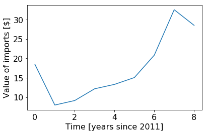
Now, with this data in hand, I actually feel like I have a reason to start assigning numbers to an outside view. Specifically, I can make an outside view prediction that the future will just follow the trajectory of the past. The physicist in me thinks that a good first guess is we can take a linear approximation of the trend by fitting a line to it, using the functional form

def outside_func(t, m, b):
    return m*t + b

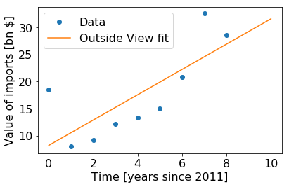
The most naive interpretation of this is to evaluate the outside_func function at t=10, which suggests that the value for 2021 will be 31.5 billion USD. However, our goal is not to predict the most likely number, but to produce a distribution. That is, how likely is each specific $y$ value. I think with the fit uncertainty we could analytically build up the probability density function $P(y)$ for the ranges of $y$ we care about. However, I think an equivalent way to do this is to just run a Monte Carlo simulation were we randomly sample from our fit parameters, and then bin the value of outside_func(t=10) that we get from the simulation.

To generate the Monte Carlo simulation, we want to plot lines that have the parameters [m,b] drawn from the distribution defined from the covariance matrix of the fit. Wikipedia gives the formula for this joint distribution given the best fit parameters and covariance matrix. This is just the formula for the multivariate normal distribution, which numpy already has a built in function to sample from. So, we can generate, for example, 1000 samples of the fit parameters in a single line of code:

fit_params_gen = np.random.multivariate_normal(popt, pcov, 1000)

where popt and pcov are the best fit parameters and covariance matrix returned from the scipy.optimize.curve_fit() function. Then, we can just plot these 1000 lines, calculate outside_func(t=10) for each of them, and build a histogram of that distribution in each of the bins selected by Foretell:

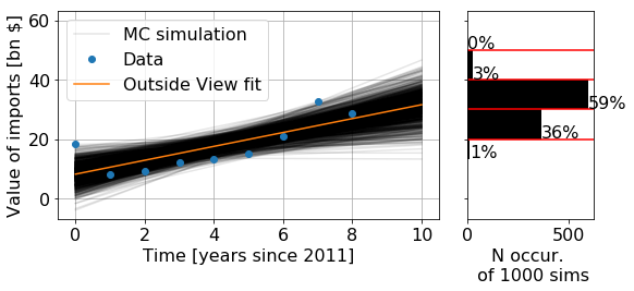
So, this gives some quantitative probabilities for a starting point. However, notice that this model puts extremely low values on some of the bins. I’m generally skeptical I should ever put 0% in a forecast, and this seems especially to be the case when the model is just curve fitting without outside information. So, my current resolution to this is to combine these values with my initial, uniform prior (which would have put 20% into each bin). I’m maybe 50% confident in this model. So, I will update these values by taking the mean of the uniform prior with the trend-fit value $(0.5 * [\text{prior}] + (1-0.5) * [\text{trend-fit value}])$, and then normalizing the resulting distribution. This gives my predicted values of {10%, 28%, 40%, 12%, 10%}.

So, now we have a sort of outside-view prior to work with. Now the goal is to continue to update these numbers as we gain more information about, e.g., the policies and economies of China and the countries it imports from. That’s beyond the scope of this post, hopefully I’ll write a follow up when I learn any of those details.